Spatial Clustering for Species Distribution Modeling
Published:
Citizen science biodiversity data can span large extents of space and time, but usually lack the structure required for building species distribution models which account for imperfect detection, i.e., occupancy models. Existing approaches of introducing this structure either throw away too much data due to strict definitions of sites and/or do not account for similarity in environmental feature space, leading to weaker downstream occupancy models. Spatial clustering algortihms from machine learning literature offer lucrative advantages over these existing approaches.
Background
Species distribution models (SDMs) aim to capture the patterns of species observations in relation to habitat characteristics. However, some species may be difficult to detect and can cause imperfect detection and false negatives. Occupancy models (MacKenzie et al., 2002) tackle this phenomenon by assuming that detection probability can be less than one, and consequently model the occupancy and detection processes separately, with the former being of higher scientific interest. Estimation of both occupancy and detection probabilities relies on repeated visits to sites over which occupancy is assumed to be fixed. While citizen science data can have large spatial and temporal coverage, they often require additional processing post hoc to introduce structure necessitated by occupancy models. Grouping together species observations to define sites for SDMs is the site clustering problem. Many potential solutions exist but they are afflicted with two primary challenges - (i) they either do not utilize all the training data provided to them to define sites, and/or (ii) they base their clustered sites on only geospatial features such as longitude and latitutude and do not account for similarity of species observation points in habitat/environmental feature space. In this post, we will see how spatial clustering algorithms remedy both of these issues and provide additional advantages in terms of better predicitve performance of downstream SDMs. We investigated these site clustering approaches on eBird data (Sullivan et al., 2014) of 31 avian species from southwestern Oregon, United States.
Ten Approaches to Site Clustering
We investigated ten candidate clustering approaches to address the site clustering problem. Their characteristics are summarized in Table 1. We include SVS for completeness but this method has known issues with parameter identifiability.
Table 1: Properties of candidate approaches according to four Yes/No questions.
| No. | Site-clustering approach | Can cluster size be >1? | Might some points be excluded? | Can clusters have points w/ diff. geospatial coords.? | Is similarity in feature space considered? |
|---|---|---|---|---|---|
| 1 | SVS | No | No | No | No |
| 2 | 1/UL | No | Yes | No | No |
| 3 | lat-long | Yes | No | No | No |
| 4 | 2to10 | Yes | Yes | No | No |
| 5 | 2to10-sameObs | Yes | Yes | No | No |
| 6 | rounded-4 | Yes | No | Yes | No |
| 7 | 1-kmSq | Yes | No | Yes | No |
| 8 | best-clustGeo | Yes | No | Yes | Yes |
| 9 | BayesOptClustGeo | Yes | No | Yes | Yes |
| 10 | DBSC | Yes | No | Yes | Yes |
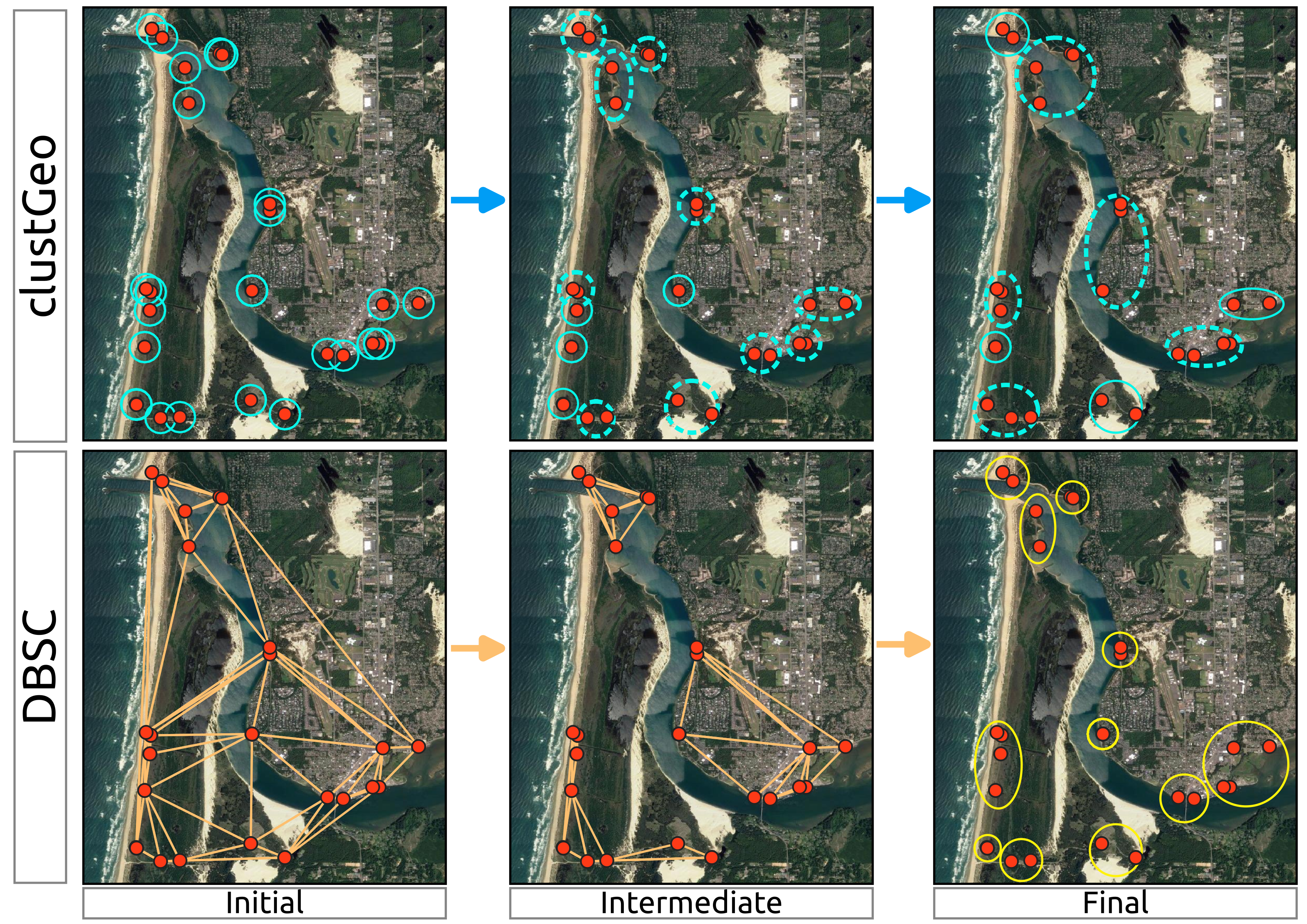
Inner workings of the two main spatial clustering algorithms - clustGeo (Chavent et al., 2018), and density based spatial clustering (DBSC) (Liu et al., 2012), are outlined in Figure 1. BayesOptClustGeo and best-clustGeo are both based on clustGeo. best-clustGeo is an oracle method which gets to optimize the clustering parameters based on test performance whereas BayesOptClustGeo selects clustering parameters by maximing the average Silhouette width of clustered points.

Figure 1: Simulated example of site formation by spatial clustering algorithms clustGeo and DBSC. eBird checklists from southwestern Oregon, United States are shown as red points. clustGeo starts off by assigning every point to its own cluster and then iteratively merges them. DBSC constructs a Delaunay Triangulation (DT) which is then split to form sub-graph DTs and then clusters.
Predictive Performance
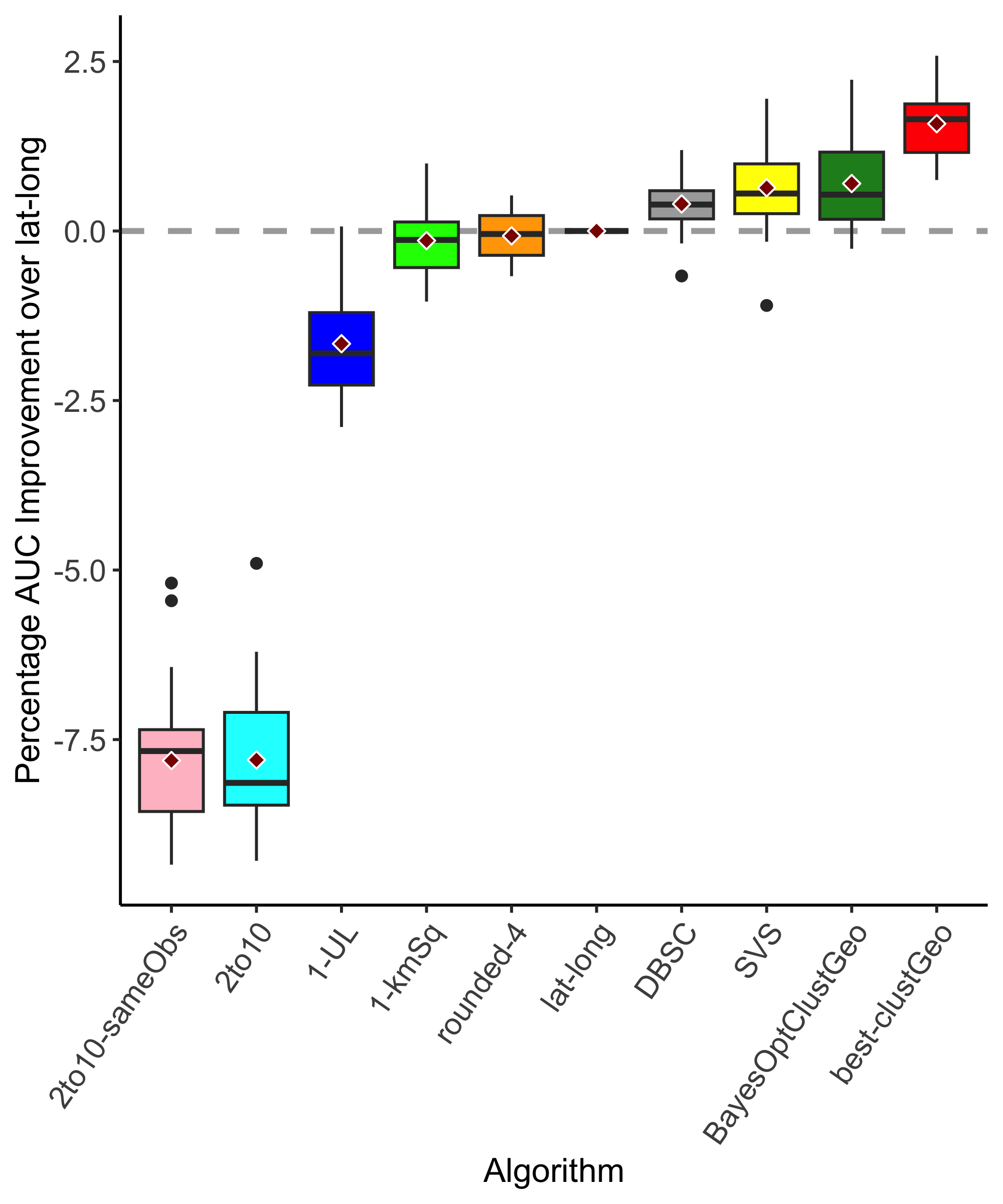
Predictive performance summarized over all species is shown in Figure 2. The main takeaways are as follows:
BayesOptClustGeo and DBSC performed the best, showing how spatial clustering leads to better downstream models compared to existing approaches.
Methods which do not factor in environmental feature space (lat-long, rounded-4, 1-kmSq) have weaker predictive performance compared to spatial clustering approaches.
Methods which discard data (2to10, 2to10-sameObs, 1-UL) trail all other methods.

Figure 2: Percentage AUC improvement over lat-long. Positive values indicate better performance than lat-long.
Occupancy Maps
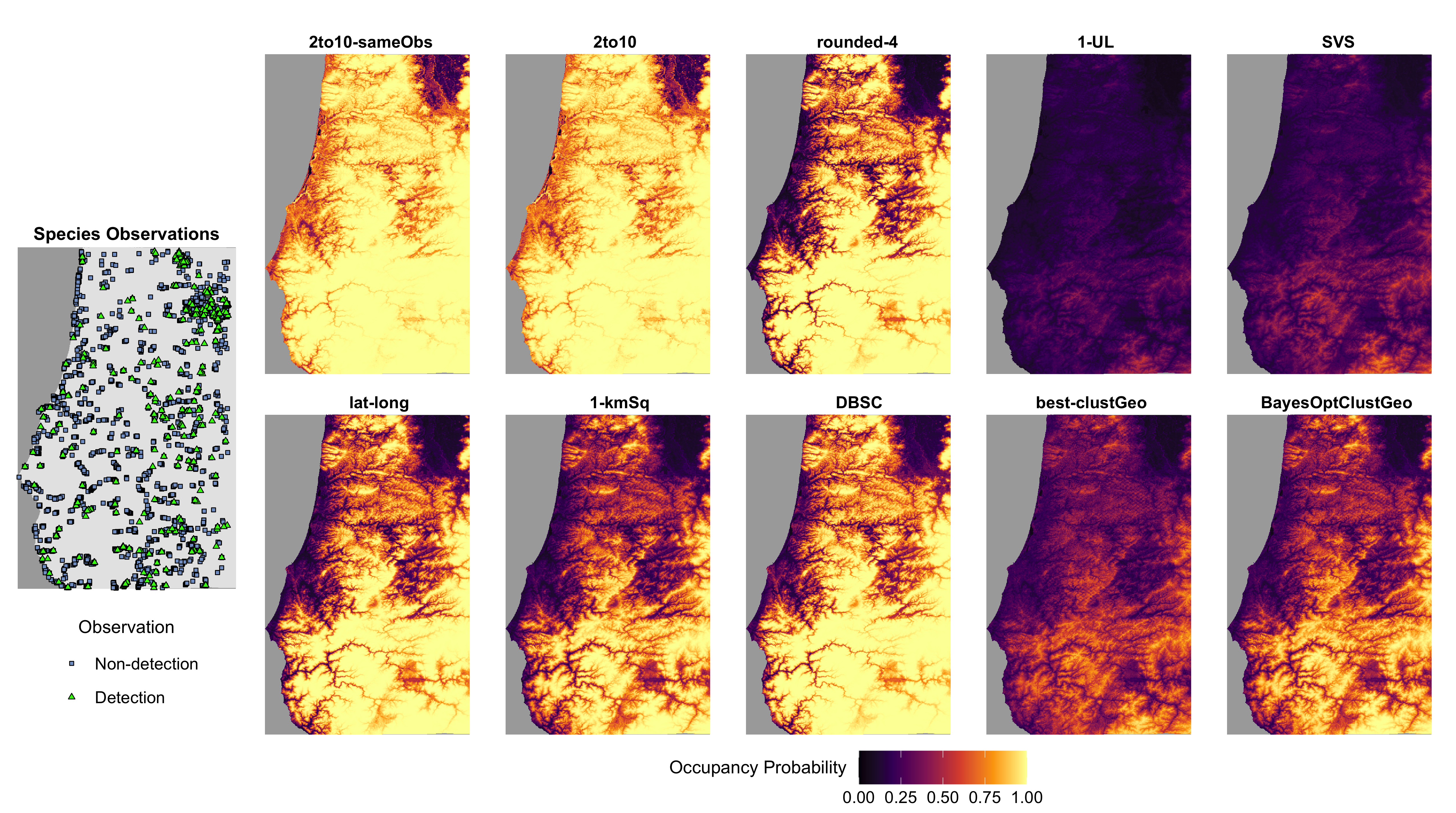
Predicted occupancy maps show the patterns of species distributions governed by the choice of site clustering approaches (Figure 3). Further expert analysis is required to assess reliability.

Figure 3: Occupancy maps of Norther Flicker (Colaptes auratus) over southwestern Oregon, United States predicted by models built on sites defined by ten clustering approaches.
References
- MacKenzie, D. I., Nichols, J. D., Lachman, G. B., Droege, S., Andrew Royle, J., & Langtimm, C. A. (2002). “Estimating site occupancy rates when detection probabilities are less than one.” Ecology, 83(8), 2248-2255.
- Sullivan, B. L., Aycrigg, J. L., Barry, J. H., Bonney, R. E., Bruns, N., Cooper, C. B., … & Kelling, S. (2014). “The eBird enterprise: An integrated approach to development and application of citizen science.” Biological conservation, 169, 31-40.
- Chavent, M., Kuentz-Simonet, V., Labenne, A., & Saracco, J. (2018). “ClustGeo: an R package for hierarchical clustering with spatial constraints.” Computational Statistics, 33(4), 1799-1822.
- Liu, Q., Deng, M., Shi, Y., & Wang, J. (2012). “A density-based spatial clustering algorithm considering both spatial proximity and attribute similarity.” Computers & Geosciences, 46, 296-309.
